Examining 
          t
          he Factors Affecting Exports Performance: Empirical Evidence 
          from Finland

Hafiz Asim; Adnan Ali Shahzad; Bilal Nafees; Muhammad Faraz Mubarak

doi:10.31384/jisrmsse/2022.20.2.5

Examining t he Factors Affecting Exports Performance: Empirical Evidence from Finland

Hafiz Asim ^1,2 , Adnan Ali Shahzad ✉ ³ , Bilal Nafees ³ , Muhammad Faraz Mubarak

⁴

1 Western Sydney University, Australia

2 University of Management and Technology, Lahore

3 University of Education, Lahore, Pakistan

4 Kaunau University of Technology, Lithuania

Abstract

Present research is an effort to diagnose the exigent determinants of the exports in Finland by using time series data from 1993-2020. The study employs vector-error correction model (VECM) by using Johansen technique to co-integration. The empirical findings of the co-integration indicate the existence of significant relationship between exports and its various determinants in the long-run. The results of VECM revealed that exchange rate and remittances are significant and positive determinants of the Finland’s exports in the long run. In the meanwhile, the impact of exchange rate and remittances is significant but negative on the exports of Finland in the short-run. On the other hand, industrial growth and corruption are incorporated in the model as exogenous factors in the short-run dynamics. The impact of industrial growth is positive and significant on the exports performance while the corruption is negatively affecting the exports of Finnish economy. The study suggests a conducive and stable exchange rate policy and control on corruption to encourage the exports.

Keywords

exports, finland, industrial growth, corruption, remittances

INTRODUCTION

The comparison of economic competitiveness is witnessed that Finland has performed very well as compared to the big and dominant economies of the world. Industrialization in Finland occurred late, and it really competed the most progressive nations after the World War-II. The present prosperity of Finland was attained late as the country remained poor and mainly agrarian as compare to its regional countries until the World War-II (Pohjola, 2003). Economic development has been considered as a main objective of every economy worldwide and economic growth is considered as essential component of economic development for any society. Among the different variables which are responsible for the growth of an economy, export is considered as a key determinant of growth as shown by Agosin (2007). A country's export of the different commodities is thought to be a foremost aspect in its social and economic development (Konya, 2006). It is said that “Finland lives on exports” as till the late 50s, about 90% of Finland’s exports were based on forest industry (Lilja, Räsänen, & Tainio, 1992). On the other hand, its industrial sector and exports base have also experienced diversification over time, particularly into machinery and metal; however, the role of forest industry was significant in the development of this economy.

The population of Finland is 5.52 million; among this 2.77 million is the labor force and unemployment rate is 7.8%. Finland’s exports of the goods and services are 35.9% of its overall gross domestic product (GDP) in 2020. Data shows that exports have a significant contribution in GDP of Finland as it is a source of foreign exchange (Oinonen & Virén, 2022). Therefore, it is important to identify and examine the determinants that have significant impact on Finnish exports over time. It will help us to determine, what explains the variations in Finnish exports’ performance over time that will enable the formulation of the policies for the improvement of its performance and finally the overall growth of the economy. Various studies have analyzed the customary determinants of exports in Finland (Bostan, Toderașcu, & Firtescu, 2018; Lupu, Petrisor, Bercu, & Tofan, 2018; Thuy & Thuy, 2019). This paper makes a significant contribution in the existing knowledge by adding industrial growth and corruption as the important factors behind the exports performance in case of Finland. Moreover, the study also gives insight to see the time varying relationships for the Finnish economy.

The empirical research on Finnish exports is not looking so attractive. The studies records are sporadic, which are mainly connected with the empirical investigation of Finnish exports and these studies covered only some regimes of post war era and have avoided using econometrics’ approaches (Haaparanta et al., 2017; Mäki-Fränti, 2017; Oinonen & Virén, 2022; Stenborg, Huovari, Kiema, & Maliranta, 2021). The originality of this paper is to employ the latest methodologies to determine various factors that affect the export performance of Finland. After ascertaining these factors, the study would be able to employ this information to estimate the effects of different policy measures that were executed by the economy. Therefore, understanding the time varying effects of different factors on exports and their implications may prove fruitful in the explanation of certain outcomes of the past policies and also in determining the optimal policy measures for the country’s economy. Consequently, the purpose of recent study is to analyse the dynamics of short and long-term effects of the various factors on Finnish exports and originate conceivable suggestions for Finland’s foreign trade. This research study will be useful for the policymakers to formulate appropriate policies with regard to the determinants of exports.

LITERATURE REVIEW

Real exchange rate as a determinant of export

The foremost variable that impacts the supply capacity of exports or the demand decision of exports is the real exchange rate (RER). It is argued that RER is crucial in determining the export growth of goods produced by a country and their competitiveness in the international market (UNCTAD, 2005). It is an essential factor that needs the government’s intentions to expand and diversify exports (Biggs, 2007).Oyejide (2007) claims that if the adjustment of RER to the actual levels is ensured, it can enhance the country’s incentives for exports and; hence, may lead to a rise in producing exportable items. While an increase in the value of local currency can deteriorate the rivalry reactions of the exports due to the reduction in price competitiveness for the export-oriented firms, devaluation of currency can boost the competitiveness of exports (Biggs, 2007) which motivates exporting activities (Oyejide, 2007).Muhammad (2014) empirically estimated the role of RER volatility on global trade and established that devaluation of exchange rate directly affects the export levels. In contrast, some research studies found RER’s negatively significant impact on the exports of various countries (Abeysinghe & Yeok, 1998; Fang & Miller, 2004). Mohamad, Nair, and Jusoff (2009) estimated the role of exchange rates and other supporting variables towards export performance of Indonesia, Malaysia, Singapore, and Thailand by applying panel data modelling. These studies determined that the appreciation of ER has a negative impact on the performance of exports.

Exchange rate and GDP as determinants of exports

Anagaw and Demissie (2012) examined the factors affecting Ethiopian exports using data from 1970-2010. The model is estimated by using VECM based on Johanson co-integration approach. The long run results have shown that export performance has been affected positively by the exchange rate, infrastructural development, RGDP, openness, and private sectors’ credit facility. While the findings of short run revealed that only the first period lag of transparency has been involved directly in enhancing the current year’s export performance.

Epaphra (2016) has examined the factors affecting Tanzania’s exports. The study employed Johansen multivariate co-integration (Johansen, 1988), Granger causality technique and VECM to estimate the model from 1966 to 2015. The results of the co-integration technique revealed the stable long-term relationship among the model’s factors. Findings show that exchange rate, trade liberalisation and per capita real GDP directly affect the Tanzanian exports’ performance. Some studies also find the significant and direct impact of ER on exports. According to them, real depreciation or undervaluation raises the profits of the tradable sector, which enhances its share in value-added domestically (Rodrik, 2008). Thuy and Thuy (2019) empirically analysed the impact of RER instability on exports. This study used quarterly data from 2000 to 2014 for Vietnam and employed the bound testing methodology. The findings indicated the negative effect of ER devaluation on exports in the short-run. Meanwhile, the impact of depreciation is positive on exports in the long-run, which is also consistent with J-curve.

Industrial production, remittances and corruption

The present study found limited literature which focused on the remittances, industrialisation and corruption as possible determinants of the exports.Vaaler (2011) revealed trade openness of home countries could be raised by increasing remittances. The author established that remittances significantly improve the level of integration of domestic economies with the rest of the world.Hien (2017) also analysed the role of remittances towards trade balance in Malaysia’s case from 1990 to 2015. The study concluded that the balance of trade is positively influenced by the inflow of remittances in Malaysia. Furthermore, the results also showed the direct relationship between RER and the trade balance.Kozo and Tetsuji (2013) argued that the long run industrial policy of an economy is a vital instrument that can diversify markets.Zalk (2014) believes that the role of industrial policy is the promotion of exports which promote competitiveness. Agosin, Alvarez, and Bravo-Ortega (2012), argued that an economy’s well-developed industrial sector could quickly sweep out competitors from the world market, as the industrial policy of the home economy helps compete with the international market.

Alternatively, institutional aspects of an economy also play a vibrant impacts on the performance of country’s exports. This can affect firm performance negatively as it raises the “un-productive” expenditures by limiting the revenues and expected returns on their investment and; hence, may influence the economy negatively (Dridi, 2013; Rosa, Gooroochurn, & Görg, 2010).Wei (1997) argued that corruption creates uncertainty as it encourages illegal activities in the export intensity of an economy, because it helps firms avoid punishments through the bribes (Olken & Pande, 2012). Some researchers also confirmed the inverse impact of corruption on firm growth and exports by using empirical data (Fisman & Svensson, 2007; Olney, 2016). Oo, Kueh, and Hla (2019), using the panel ARDL approach for ASEAN economies from 2000–2015, found the inverse relationship between the rate of interest and exports in the short and long run. The study concluded that interest rate stability enhances the countries’ export performance. (Oliveira, Jegu, & Santos, 2020) analysed export diversification and its factors in Brazil’s various economic regions from 2003 to 2013 by employing the generalised method of moments. Findings showed that the exports are more diversified in the Southeastern states compared to the Northeastern region, and divergence in the Centralwest region started in 2006.

The role of the above discussed literature is worthwhile in investigating the export delineation of the economies. There are many studies which have estimated the factors that affecting exports in the developing economies (David, 2013; Keho, 2015; Uysal & Mohamoud, 2018). In contrast, the research on the subject under discussion for the developed world is qualitative as we could hardly found any research study on the export conditions of high income countries like Finland by employing the most appropriate methodology. Hence, the rationale behind the present study is to determine the exigent determinants of exports for Finnish economy by using time series data.

METHODOLOGY

The present paper has collected time series annual data from WDI (2021). The data on all the variables have been collected from 1993 to 2020. Only the data on the variable of corruption has been composed from the International Country Risk Guide (ICRG, 2020). This study uses a dynamic time series regression analysis to build a model for investigating the determinants of exports in Finland, which permits us to handle the non-stationary series more effectively. Most economic models are dynamic in nature, which is expected for the policy changes that have long-run impacts and persist in the future. Thus, the dynamic version of the model explains the impacts of independent variables over time. For the reasons mentioned above, most empirical studies have moved from static modelling to dynamic regression methods (Headey, 2013). Therefore, as explained in the above section, we have modelled the exports of goods and services (as a % of GDP) as a function of its determinants. Hence, according to the relationship among the remittances, exchange rate, industrial growth, corruption and exports as explained in the preceding section, the model is specified as follows:

X G D P_{t} = f (R E E R_{t}, P R E M G D P_{t}, I G_{t}, C R P_{t})

The econometric version of the above model is given as following:

X G D P_{t} = β_{0} + β_{1} R E E R_{t} + β_{2} P R E M G D P_{t} + β_{3} I G_{t} + β_{4} C R P_{t} + μ_{t}

The study has used the following semi-log form of the above model:

l n X G D P_{t} = β_{0} + β_{1} l n R E E R_{t} + β_{2} l n P R E M G D P_{t} + β_{3} I G_{t} + β_{4} l n C R P_{t} + μ_{t}

Here the subscript t represents the time, while the variables’ description is presented in Table 1. It is essential to mention that the industrial growth and corruption index are included as exogenous variables in the model. Semi-log model is developed in Equation 3 because industrial value added is in growth form and other variables are not in growth form; hence, the study has taken a log of all other variables; however, the results have been interpreted accordingly. Different studies confirmed that the results of models in log form are considered more reliable in contrast to the models findings in a simple form (Ehrlich, 1996; Layson, 1983).

Table 1: Variables Description and Data Sources

Variable	Representation	Description	Transformation	Data Sources
Exports	${l n X G D P}_{t}$	Exports of Goods & Services as a share of GDP	ln(Exports/GDP)	WDI; The World Bank, 2020
Exchange Rate	${l n R E E R}_{t}$	Real Effective Exchange Rate Index	ln(Real Effective Exchange Rate Index)	WDI; The World Bank, 2020
Remittances	${l n P R E M G D P}_{t}$	Personal Remittances Received	ln(Personal Remittances Received/GDP)	WDI; The World Bank, 2020
Industrial Growth	${I G}_{t}$	Industrial value added (annual % growth)	Industrial value added/GDP	WDI; The World Bank, 2020
Corruption	${l n C R P}_{t}$	Corruption Index	Ln(Corruption Index)	ICRG (2020)

Empirical Findings

Correlation and variance inflation factor (VIF) matrices were calculated at the very outset to test the multi-collinearity. The correlation matrix and matrix of VIF were estimated to detect the severity of multi-collinearity in our model. The findings are portrayed in Table 2 and Table 3, respectively.

Table 2: Correlation matrix

	LNEX	LNREER	LNPREM	IG	LNCRP
LNEX	-	-	-	-	-
LNREER	-0.8698	-	-	-	-
LNPREM	0.8079	-0.8219	-	-	-
IG	0.1855	-0.0422	0.0331	-	-
LNCRP	-0.2254	0.5178	-0.4201	0.1804	-

Source: Estimated by the authors

Table 3: Matrix of variance inflation factor

	LNEX	LNREER	LNPREM	IG	LNCRP
LNEX	-	-	-	-	-
LNREER	4.10765405	-	-	-	-
LNPREM	2.87937501	3.08185	-	-	-
IG	1.03563651	1.00178	1.0011	-	-
LNCRP	1.05352448	1.36634	1.21431	1.0336389	-

Source: Estimated by the authors

The empirical findings in Table 3 indicates that the magnitude of VIF among all the explanatory variables is less than 10, which depicts no significant relationship among the regressors. Therefore, it can be postulated that there is an absence of multi-collinearity in the data. Moreover, to analyse the trends and features of data, the graphical representation is presented in Figure 1.

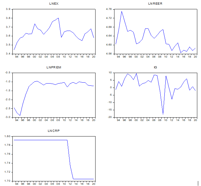
https://typeset-prod-media-server.s3.amazonaws.com/article_uploads/581fd815-38c5-4ece-b4d9-9401a814dff6/image/6e599603-3aec-4eac-9ae9-3fdc26c9c8c1-ucapture-adnan.png — Figure 1: *Graphical representation of the variables of the model.*

Graphical analysis is the first step to comprehend the nature and trends of time series data. It also helps to analyse data features such as trends and direction. Moreover, the graphical analysis of time series data helps to observe the structural breaks and presence of unit roots in the series. In graphical analysis, the data, for all the variables in the model, is presented in natural logarithmic form, demonstrating that the key variables, lnXGDP and lnPREMGDP reveal a very smart rise but with very little volatile behaviour. On the other hand, lnREER is showing a descending but linear trend, whereas the data of corruption index (lnCRP) is showing a moderately smoother behavior with a sudden decreasing trend. In contrast, industrial growth (IG) series is comparatively volatile. The visual observation of the graphs postulates that the majority of the variables comprised in our study have a unit root problem; therefore, we are unable to apply the ordinary least squares (OLS) technique in this situation as series having unit root may create spurious results, if analysed with OLS (Asim & Akbar, 2019).

Moreover, the unit root problem in the data series and the stationarity level determine the model’s estimation method. Therefore, the next portion is earmarked to test the possible existence of unit root in our time series data. This is done with the help of ADF and PP tests of stationary. The relevant results are presented inTable 4.

Table 4: Results of unit root tests

			ADF Test at Level
Variables	t-statistic	p-value	Lags (k)	Decision (d)	Variables	t-statistic	p-value	Lags (k)	Decision (d)
LNEX	-3.0215	0.145	0	Non-Stationary	LNEX	-5.5816	0.0006	0	Stationary
LNREER	-1.9524	0.3048	0	Non-Stationary	LNREER	-4.5339	0.0016	0	Stationary
LNPREM	-2.1921	0.2134	0	Non-Stationary	LNPREM	-3.4647	0.0176	0	Stationary
IG	-2.0133	0.2796	2	Non-Stationary	IG	-4.331	0.0025	2	Stationary
LNCRP	-0.8239	0.7954	1	Non-Stationary	LNCRP	-3.3904	0.0212	1	Stationary
	Phillips Perron Test at Level
Variables	t-statistic	p-value	Lags (k)	Decision (d)	Variables	t-statistic	p-value	Lags (k)	Decision (d)
LNEX	-3.0053	0.1491	1	Non-Stationary	LNEX	-5.8310	0.0003	3	Stationary
LNREER	-1.9524	0.3048	0	Non-Stationary	LNREER	-7.9604	0	11	Stationary
LNPREM	-2.1921	0.2134	0	Non-Stationary	LNPREM	-3.5364	0.015	2	Stationary
IG	-0.2743	0.5778	16	Non-Stationary	IG	-19.911	0	16	Stationary
LNCRP	-0.4085	0.8942	1	Non-Stationary	LNCRP	-3.2593	0.0277	3	Stationary

Source: Estimated by authors

Note: k = Optimum lag length; and I(d) = Order of integration = 1

The null hypothesis of both ADF and PP unit root tests indicates that the series has a unit root, whereas the alternate hypothesis shows that the series doesn’t have a unit root issue. The empirical findings of both unit root tests show that we fail to reject null hypothesis of unit root at a level in all the series. The results indicate that we remained successful in rejecting the null hypothesis of unit root at first difference. It means all the variables are integrated in order 1, i.e. I(1). Therefore, the next step is to test the co-integration between the variables of the model by employing Johansen multivariate co-integration approach (Johansen, 1988). Before applying the Johansen multivariate co-integration technique, we check the lag length based on the lag length criteria presented by AIC and SBC. The findings, given in Table 5, indicate that the optimal lag length is three. The findings of Johansen multivariate co-integration are placed inTable 6.

Table 5: Lag Length Criterion

Lag	LogL	LR	FPE	AIC	SC	HQ
0	52.2065	NA	7.40E-06	-3.3005	-3.0150	-3.2132
1	129.6669	127.2563	5.63E-08	-8.1905	-7.4768	-7.9723
2	143.3931	19.6088	4.17E-08	-8.5281	-7.3862	-8.1790
3	161.7802	22.3272*	2.32e-08*	-9.1986*	-7.6285*	-8.7186*

Source: Estimated by the authors

Note: * indicates lag order selected by the criterion

Table 6: Multivariate Co-integration Approach

	Trace Test
Null Hypothesis	Alternative Hypothesis	Trace Test	Critical value at 5% Significance Level
r=0	r=1	88.1674	29.7971
r≤1	r=2	32.6337	15.4947
r≤2	r=3	8.3095	3.8415
Maximum Eigen Value Test
Null Hypothesis	Alternative Hypothesis	Maximum Eigen Value Test	Critical value at 5% Significance Level
r=0	r=1	55.5336	21.1316
r≤1	r=2	24.3242	14.2646
r≤2	r=3	8.3095	3.8415

Source: Estimated by author.

Note: r represents a number of co-integrating vectors, * denotes rejection of the null hypothesis at the 5% significance level.

Both trace and maximum eigenvalue test indicate 3 co-integrating equations at 5% significance. We use trace and maximum eigenvalue tests to establish co-integration. The results of both test statistics show three co-integrating vectors at 5% significance level. So, the study revealed the existence of co-integration between exports and its determinants included in the case of Finland. After establishing the co-integration, VECM has been applied to estimate long-run and short-run coefficients. The empirical findings of VECM are portrayed in Table 7.

Normalised Long-run Coefficients

The results of VECM show that the real effective exchange rate and personal remittances significantly and directly impact exports in the long-run in the Finnish economy. The coefficient of the REER is found to be 43.15749 and significant, which shows that an increase in the real effective exchange rate by 1%, in the long-run, will significantly increase exports of goods and services by 43.15749% in Finland. It means that the rise in the real effective exchange rate causes the depreciation of the local currency, making the exportable commodities cheap and; hence, resulting in the growth of the export performance of Finland. This result is consistent with the Marshal-learner condition, which says that the exports performance of a country improves with the upward movements in the REER in the long run (Anagaw & Demissie, 2012; Epaphra, 2016; Ramana, 2022; Tomoiaga & Silaghi, 2022).

Whereas the relationship between the exports and remittances is also found to be positive and significant. It means that, in the long run, exports are increased with the rise in the remittances received by the Finnish economy. The coefficient of remittances is turned to be 1.8960 and significant, which reveals that if remittances increase by 1%, then it will significantly result in a rise in exports by 1.8960%. The finding is consistent with (Hien, 2017; Regmi, 2022; Vaaler, 2011). The relative impact of the real effective exchange rate is more significant than the relative influence of the remittances on Finnish exports. This means that the REER is the most important factor that may affect Finnish exports in the long-run.

Table 7: Normalized long-run coefficients

Independent Variables

Coefficients

Decision

lnREERt

43.15749

(3.9378)

[-10.9598]

Significant

lnPREMGDPt

1.8960

(0.3074)

[-6.1675]

Significant

193.8023

Dependent variable: lnXGDPt

Source: Estimated by the author.

Notes: Standard errors arereported in ( ) and t-statisticsin [ ].

Table 8: Adjusted short-run coefficients

Independent Variables	Coefficients	Decision
ΔlnXGDPt (-1)	0.200997 (0.15148) [1.32690]	Insignificant
ΔlnREERt (-1)	-0.665714 (0.23619) [-2.81856]	Significant
ΔlnPREMGDPt (-1)	-0.167125 (0.05074) [-3.29402]	Significant
ΔIGt (-1)	0.009097 (0.00167) [ 5.45163]	Significant
ΔlnCRPt (-1)	-0.713912 (0.31967) [-2.23326]	Significant
C	1.247367 (0.56245) [ 2.21772]	Significant
Ectt-1	-0.026302 (0.00728) [-3.61154]	Significant

Dependent Variable: ΔlnXGDPt

Source: Estimated by author.

Notes: Standard errors arereported in ( ) and t-statisticsin [ ].

Adjusted short-run coefficients

After highlighting the long-run coefficients, we will now discuss the adjusted short-run coefficients presented in Table 8. The coefficient of first lagged exports is positive but insignificant in the short-run, and the REER coefficient is negative and significant in the short-run. It shows that a 1% rise in the real effective exchange rate will result in a 0.6657% decrease in exports in the Finnish economy in the short-run.Abeysinghe and Yeok (1998); Fang and Miller (2004); Mohamad et al. (2009) also found a similar relationship between the exchange rate and export performance of different countries. Whereas the coefficient of remittances is turned to be -0.1671 and significant, which reveals that if remittances increase by 1%, then it will significantly result in a decline in exports by 0.1671% in the short-run.Azizi (2021) also established a similar relationship between remittances and exports in the developing countries.

Moreover, industrial growth and corruption are encompassed in the econometric model as the exogenous variables. The coefficient of industrial growth is turned to be 0.00909, which shows a direct and significant impact of industrial growth on Finnish exports. It indicates that Finnish exports rise by 0.00909% for every percent increase in industrial value added in the short-run. Agosin et al. (2012); Zalk (2014) also varified the similar relationship. In contrast, the impact of corruption is negative and significant on Finnish exports in short-run. It designates that if corruption increases by 1%, Finnish exports will decrease by 0.7139%. These findings can also be verified from previous researches (Dridi, 2013; Fisman & Svensson, 2007; Olney, 2016; Rosa et al., 2010; Wei, 1997).

In the long-run, the adjustment factor for exports is negative, significant and less than one. It indicates a long-term stable relationship between exports and real effective exchange rate, remittances; industrial value added growth and corruption for Finland’s economy. Its value is -0.0263, which shows that the speediness of modification towards the equilibrium is 2.63% per year in case of any shock, as the study has used annual time series data, and it would take almost 38 years for this adjustment.

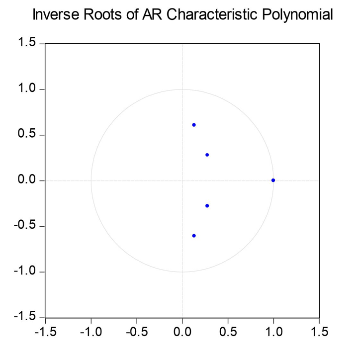
To check the reliability of estimated results, we have applied some diagnostic tests (Joint Jarque–Bera-normality test, heteroskedasticity test, serial correlation LM test, and AR root test) to the estimated model. The results are given in Table 9. The estimated values of normality tests like heteroskedasticity and serial correlation tests were insignificant, showing the acceptance of these tests’ null hypothesis. It means that the residual term of the estimated model follows a normal distribution, the variance of the residual term is homoscedastic, and there is no serial correlation problem in the estimated model. After checking the model’s reliability, we applied the AR root test to check the time variant stability of our estimated coefficients. The graph of the AR-root test presented in Table 9 shows that all of the coefficients are structurally stable over time. So, it can be concluded that our estimated model is reliable and structurally stable.

Table 9: Diagnostic Tests

Test

Values

VEC Residual Normality Test: Joint Jarque–Bera Test

3.8253

(0.7003)

VEC residual serial correlation LM test

For lag = 1 12.9636 (0.1643)

For lag = 2 4.7408 (0.8563)

VEC residual heteroskedasticity test:

Joint chi-square test

560.6124

(0.3233)

https://typeset-prod-media-server.s3.amazonaws.com/article_uploads/581fd815-38c5-4ece-b4d9-9401a814dff6/image/85b9143e-ecb4-4d99-b3a3-7b3df22d0518-ufig-2.png — **Figure 2: Stability test: AR-roots graph**

CONCLUSION AND POLICY RECOMMENDATIONS

This paper analyses the export performance of Finland by using the annual data of 1993 to 2020. Time series estimation methods are used to analyse the determinants of Finnish export performance over time. To establish the long run stable association among the study variables, the Johansson co-integration technique is employed, and its results confirm the existence of long run relationship among the series of the assessed model. The pragmatic results of the model on the determinants of Finland’s exports show that REER and personal remittances are positive and significant long run determinants of Finland’s exports. In contrast, the impact of real effective exchange rate and remittances is negative and significant in short-run. On the other hand, industrial growth and corruption are included in the model as the exogenous variables in the dynamics of the short run. Industrial growth has a significant and direct impact on exports performance, while corruption negatively affects the exports of Finnish economy. The empirical findings suggest that a stable and conducive policy for the exchange rate should be ensured. The government has to control corruption, and further depreciation of the local currency should be allowed in the long-run to boost more exports.

Conflict of interest statement

The authors declare no conflict of interests.

[1] Pohjola, M . 2003. Olemmeko maailman parhaimmistoa? Kansallisen kilpailukykymme puntarointia. In: Talouden tutkimus ja päätöksenteko. Kirjoituksia rakennemuutoksesta, kasvusta ja talouspolitiikasta (163-181). (pp. 163-181) TALOUSTIETO OY

[2] Agosin, M R . 2007. Export diversification and growth in emerging economies. 233:559–562.

[3] Konya, L . 2006. Exports and Growth: Granger Causality Analysis on OECD Countries with a Panel Data Approach. Economic Modelling 23:978–992.

[4] Lilja, K, Räsänen, K & Tainio, R . 1992. A dominant business recipe: the forest sector in Finland. European business systems: Firms and market in their national contexts 137–154.

[5] Oinonen, Sami & Virén, Matti E E . 2022. Why is Finland lagging behind in export growth? BoF Economics Review (5).

[6] Bostan, I, Toderașcu, C & Firtescu, B N . 2018. Exchange rate effects on international commercial trade competitiveness. Journal of Risk and Financial Management 11(2):19.

[7] Lupu, D, Petrisor, M B, Bercu, A & Tofan, M . 2018. The impact of public expenditures on economic growth: A case study of Central and Eastern European countries. Emerging markets finance and trade 54(3):552–570.

[8] Thuy, V N T & Thuy, D T T . 2019. The impact of exchange rate volatility on exports in Vietnam: A bounds testing approach. Journal of Risk and Financial Management 12(1):6.

[9] Haaparanta, P, Tamminen, S, Heikkinen, P M S, Aunesluoma, J, Hakkala, K Nilsson, Kiviluoto, J & Rissanen, A . 2017. 100 vuotta pientä avotaloutta: Suomen ulkomaankaupan kehitys, merkitys ja näkymät. .

[10] Mäki-Fränti, P . 2017. Finland struggling to defend its market share on rapidly expanding markets. .

[11] Stenborg, M, Huovari, J, Kiema, I & Maliranta, M . 2021. Productivity and competitiveness in Finland Which factors affect competitiveness? Why do we need it. valtiovarainministeriö 978–952.

[12] , UNCTAD. 2005. Determinants of Export Performance: Developing Countries in International Trade. Trade and Development Index 49–79.

[13] Biggs, T . 2007. Assessing export supply constraints: methodology, data, measurement. AERC Research Project on Export Supply Response Capacity Constraints in Africa.

[14] Oyejide, T A . 2007. African Trade, Investment and Exchange Rate Regimes and Incentives for Exporting. AERC Research Project on Export Supply Response Capacity .

[15] Muhammad, Z . 2014. Macroeconomic Relationships between Exchange Rate Instability, Exchange Volatility, Trade and Economic Growth Variables: The case of Pakistan. Journal of Economics and Sustainable Development 5(13).

[16] Abeysinghe, T & Yeok, T L . 1998. Exchange rate appreciation and export competitiveness. The case of Singapore. Applied economics 30(1):51–55.

[17] Fang, W & Miller, S . 2004. Exchange Rate Depreciation and Exports: The Case of Singapore. Economics Working Paper .

[18] Mohamad, S, Nair, M & Jusoff, K . 2009. Exchange rates and export competitiveness in selected ASEAN economies. International Business Research 2(2):156–166.

[19] Anagaw, B K & Demissie, W M . 2012. Determinants of export performance in Ethiopia: VAR model analysis. Journal of Research in Commerce & Management 2(5):94–109.

[20] Epaphra, M . 2016. Determinants of export performance in Tanzania. Journal of Economics Library 3(3):470–487.

[21] Johansen, S . 1988. Statistical analysis of co-integration vectors. Journal of Economic Dynamics and Control 12:231–254.

[22] Rodrik, D . 2008. The real exchange rate and economic growth. Brookings papers on economic activity 2008(2):365–412.

[23] Vaaler, P M . 2011. Immigrant remittances and the venture investment environment of developing countries. Journal of International Business Studies 42(9):1121–1149.

[24] Hien, N P . 2017. The impact of remittance on trade balance: The case of Malaysia. Journal of Economics and Public Finance 3(4):531–540.

[25] Kozo, K & Tetsuji, O . 2013. Effects of Industrial Policy on Productivity: The case of import quota removal during postwar Japan. The Research Institute of Economy. Trade and Industry 1–35.

[26] Zalk, N . 2014. Industrialisation and Industrial Policy. Portfolio Committee on Trade & Industry 1–18.

[27] Agosin, M R, Alvarez, R & Bravo-Ortega, C . 2012. Determinants of export diversification around the world: 1962-2000. The World Economy 35(3):295–315.

[28] Rosa, D De, Gooroochurn, N & Görg, H . 2010. Corruption and productivity firm-level evidence from the BEEPS survey (No. 5348) Policy Research Working Paper .

[29] Dridi, M . 2013. Corruption and economic growth: the transmission channels. Journal of Business Studies Quarterly 4(4):121–152.

[30] Wei, S J . 1997. Why is corruption so much more taxing than tax? Arbitrariness kills. National Bureau of Economic Research .

[31] Olken, B A & Pande, R . 2012. Corruption in developing countries. Annu. Rev. Econ 4(1):479–509.

[32] Fisman, R & Svensson, J . 2007. Are corruption and taxation really harmful to growth? Firm level evidence. Journal of development economics 83(1):63–75.

[33] Olney, W W . 2016. Impact of corruption on firm-level export decisions. Economic Inquiry 54(2):1105–1127.

[34] Oo, T, Kueh, J & Hla, D T . 2019. Determinants of Export Performance in ASEAN Region: Panel Data Analysis. International Business Research 12(8):1–14.

[35] Oliveira, H C D, Jegu, E & Santos, V E . 2020. Dynamics and determinants of export diversification in Brazil from 2003 to 2013. Economia e Sociedade 29:29–51.

[36] David, B . 2013. Competitiveness and determinants of cocoa exports from Ghana. International Journal of Agricultural Policy and Research 1(9):236–254.

[37] Keho, Y . 2015. Foreign Direct Investment, Exports and Economic Growth: Some African Evidence. Journal of Applied Economics & Business Research 5(4).

[38] Uysal, O & Mohamoud, A S . 2018. Determinants of Export Performance in East Africa Countries. Chinese Business Review 17(4).

[39] Headey, D D . 2013. Developmental drivers of nutritional change: a cross-country analysis. World Development 42:76–88.

[40] Layson, S . 1983. Homicide and deterrence: Another view of the Canadian time-series evidence. Canadian Journal of Economics 52–73.

[41] Ehrlich, I . 1996. Crime, punishment, and the market for offenses. Journal of economic perspectives 10(1):43–67.

[42] Asim, H & Akbar, M . 2019. Sectoral growth linkages of agricultural sector: Implications for food security in Pakistan. Agricultural Economics 65(6):278–288.

[43] Ramana, F . 2022. Marshall-lerner condition pada perdagangan indonesia-tiongkok. Buletin Ilmiah Litbang Perdagangan 16(1):59–78.

[44] Tomoiaga, E & Silaghi, M I Pop . 2022. Testing the Marshall-Lerner condition for Romania. Theoretical & Applied Economics 29(1).

[45] Regmi, R H . 2022. Remittances and trade balance: A new transfer problem. Remittances Review 7(1):3–19.

[46] Azizi, S . 2021. Impacts of Remittances on Exchange Rates And Net Export. Global Economy Journal 21(02):2150006.